«统计学完全教程»笔记:第2章.随机变量
随机变量
掌握各种分布。
随机变量是一个从样本空间到实数的函数。
输入:一个样本点 输出:一个实数
至于随机变量的值含义,则完全是人根据需要设置的。比如可以规定为两个骰子点数的和,点数的积,乃至点数对应的上星期某一天有没有下雨。
随机变量是指变量的值无法预先确定仅以一定的可能性(概率)取值的量。
离散随机变量:如果随机变量的输出能够被一一列举,则这种随机变量是离散的。
我们把离散型随机变量(的输出)作为键,把这个输出的概率作为值,则可以得到随机变量的分布律 $P \{X = x_i\}$。
分布函数:
$$F(x) = P \{X \leq x\}, x \in \mathbb{R} $$通过分布函数,可以求 $X$ 在任意区间取值的概率:
$$ \begin{aligned} P\left\{x_{1}累积分布函数(cumulative distribution function, or CDF),简称 分布函数 是一个从 $\mathbb{R} \to [0,1]$ 的映射,用于表示随机变量概率在 $(-\infty , x)$ 的累积。
$$ F_X(x) = P(X \leq x) $$CDF 必须满足的条件:
-
F 不减
-
F 是规范的: $\lim*{x\to-\infty} F(x) = 0 $ 且 $\lim*{x\to\infty} F(x) = 1 $
-
F 右连续
概率质量函数
概率质量函数 (probability function or probability mass function,PMF):
$F_X(x) = \mathbb{P}(X = x)$
PMF 和 CDF 的关系:
$F_{X}(x)=\mathbb{P}(X \leq x)=\sum_{x_{i} \leq x} f_{X}\left(x_{i}\right)$
对于连续随机变量:
$$ \mathbb{P}(a【例子】均匀 (0,1) 分布:
pdf:
$$ f_{X}(x)= \begin{cases}1 & \text { for } 0 \leq x \leq 1 \\ 0 & \text { otherwise. }\end{cases} $$cdf:
$$ F_{X}(x)= \begin{cases}0 & x<0 \\ x & 0 \leq x \leq 1 \\ 1 & x>1\end{cases} $$figure:
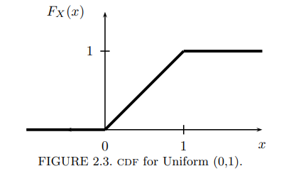
【引理】设 F 是 X 的 CDF,则
-
$\mathbb{P}(X=x)=F(x)-F\left(x^{-}\right)$, 其中, $F\left(x^{-}\right)=\lim _{y \uparrow x} F(y)$.
-
$\mathbb{P}(x
-
$\mathbb{P}(X>x)=1-F(x)$
-
如果 $X$ 是连续的, 则
$q \in [0,1]$
$\inf $ 下确界
$p = \frac{1}{4}$ 第一分位数 (first quartile) $p = \frac{1}{2}$ 第二分位数,中位数 (median) $p = \frac{3}{4}$ 第三分位数 (third quartile)
X,Y 同分布(equal in distribution): $F_X(x) = F_Y(x)$ ,记为
$$ X \stackrel{d}{=} Y $$X,Y 同分布,不代表 X = Y
概率密度函数
简称 PDF,它的积分就是 CDF。PDF 描述随机变量函数值,在某点附近的可能性。
定义:
$$ \forall -\infty其中:
-
$x$:是随机变量 $X$ 的特定函数值
-
$F_X(x)$:是 $x$ 的 CDF
则 $f_X(x)$ 是 $X$ 的概率密度函数。
下面是正态分布的 PDF/CDF Figure:

独立随机变量
Two random variables $X$ and $Y$ are independent if, for every $A$ and $B$,
$$ \mathbb{P}(X \in A, Y \in B) = \mathbb{P}(X \in A) \mathbb{P}(Y \in B) $$We write $X \text{ ⫫ } Y$.
In principle, to check whether $X$ and $Y$ are independent we need to check the equation above for all subsets $A$ and $B$. Fortunately, we have the following result which we state for continuous random variables though it is true for discrete random variables too.
Theorem 3.30. Let $X$ and $Y$ have joint PDF $f_{X, Y}$. Then $X \text{ ⫫ } Y$ if and only if $f_{X, Y}(x, y) = f_X(x) f_Y(y)$ for all values $x$ and $y$.
The statement is not rigorous because the density is defined only up to sets of measure 0.
The following result is helpful for verifying independence.
Theorem 3.33. Suppose that the range of $X$ and $Y$ is a (possibly infinite) rectangle. If $f(x, y) = g(x) h(y)$ for some functions $g$ and $h$ (not necessarily probability density functions) then $X$ and $Y$ are independent.
Multivariate Distributions and IID Samples
随机向量:Let $X = (X_1, \dots, X_n)$ where the $X_i$’s are random variables. We call $X$ a random vector.
Let $f(x_1, \dots, x_n)$ denote the PDF. It is possible to define their marginals, conditionals, etc. much the same way as in the bivariate case. We say that $X_1, \dots, X_n$ are independent if, for every $A_1, \dots, A_n$,
$$ \mathbb{P}(X_1 \in A_1, \dots, X_n \in A_n) = \prod_{i=1}^n \mathbb{P}(X_i \in A_i) $$独立同分布 It suffices to check that $f(x_1, \dots, x_n) = \prod_{i=1}^n f_{X_i}(x_i)$. If $X_1, \dots, X_n$ are independent and each has the same marginal distribution with density $f$, we say that $X_1, \dots, X_n$ are IID (independent and identically distributed).
We shall write this as $X_1, \dots, X_n \sim f$ or, in terms of the CDF, $X_1, \dots, X_n \sim F$. This means that $X_1, \dots, X_n$ are independent draws from the same distribution. We also call $X_1, \dots, X_n$ a random sample from $F$.
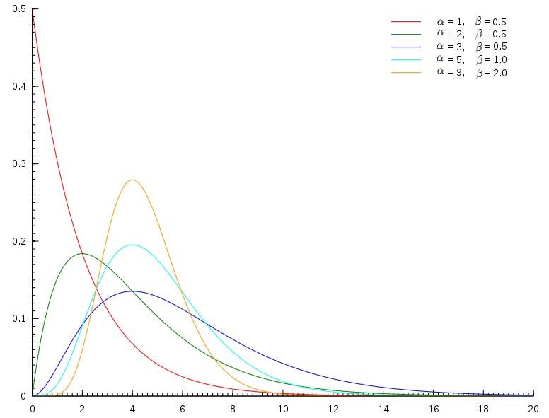
常见的分布
Point Mass Distribution
记号:$X\sim \delta_a$
\mathbb{P}(X = a) = 1
PDF:
$$ F(x)= \begin{cases}0, & xDiscrete Uniform Distribution $$ f(x)= \begin{cases}1 / k, & x=1, \cdots, k \\ 0, & \text { elsewhere }\end{cases} $$称离散随机变量 $X$ 在 $\{1, \cdots, k\}$ 上服从均匀分布.
Bernoulli Distribution (0-1 Distribution)
X 表示硬币的正反。 $\mathbb{P}(X=1)=p$ and $\mathbb{P}(X=0)=1-p$ for some $p \in[0,1] .$
记号: $X \sim \operatorname{Bernoulli}(p)$.
概率函数:$f(x)=p^{x}(1-p)^{1-x}$ for $x \in\{0,1\}$.
| X | 0 | 1 |
|---|---|---|
| px | 1-p | p |
Binomial Distribution
$$ \mathbb{P}(X \mid_{x = k}) = {n \choose k} p^k (1 - p)^{n-k} $$设硬币正面概率 $p$ for some $0 \leq p \leq 1$.
投掷 $n$ times,设 $X$ 为正面次数.
记号:$X \sim \operatorname{Binomial}(n, p)$
$f(x)=\mathbb{P}(X=x)$
$$ f(x)= \begin{cases}\left(\begin{array}{l} n \\ x \end{array}\right) p^{x}(1-p)^{n-x} & \text { for } x=0, \ldots, n \\ 0 & \text { otherwise }\end{cases} $$二项式随机变量的性质:
If $X_{1} \sim \operatorname{Binomial}\left(n_{1}, p\right)$ and $X_{2} \sim \operatorname{Binomial}\left(n_{2}, p\right)$ then $X_{1}+X_{2} \sim \operatorname{Binomial}\left(n_{1}+n_{2}, p\right)$.
二项分布的期望和方差:
$$ \mathbb{E}(X) = \lambda = np \quad \mathbb{V}(X) = np(1-p) $$Geometric Distribution
在几何分布中,随机变量 $X$ 表示投硬币第一次正面出现所经历的次数。
$X$ has a geometric distribution with parameter $p \in(0,1)$, written $X \sim \operatorname{Geom}(p)$, if
$$ \mathbb{P}(X=k)=p(1-p)^{k-1}, \quad k \geq 1 $$We have that
$$ \sum_{k=1}^{\infty} \mathbb{P}(X=k)=p \sum_{k=1}^{\infty}(1-p)^{k}=\frac{p}{1-(1-p)}=1 $$Think of $X$ as the number of flips needed until the first head when flipping a coin.
几何分布的推导:
设硬币正面出现的概率是 $p$。求 $E(X)$,$V(X)$。
$\mathbb{E}(X) = \dfrac{1}{p}$
应该也可以用矩生成函数进行推导。我试了一下,带 $e$ 级数求和做不来😂,等我问问班上的大佬。
Poisson Distribution
$$ \mathbb{P}(X \mid_{x = k}) =\frac{\lambda^k e^{-\lambda}}{k!} $$$X$ has a Poisson distribution with parameter $\lambda$, written $X \sim \operatorname{Poisson}(\lambda)$ if
$$ f(x)=e^{-\lambda} \frac{\lambda^{x}}{x !} \quad x \geq 0 $$Note that
$$ \sum_{x=0}^{\infty} f(x)=e^{-\lambda} \sum_{x=0}^{\infty} \frac{\lambda^{x}}{x !}=e^{-\lambda} e^{\lambda}=1 $$The Poisson is often used as a model for counts of rare events like radioactive decay and traffic accidents. If $X_{1} \sim \operatorname{Poisson}\left(\lambda_{1}\right)$ and $X_{2} \sim \operatorname{Poisson}\left(\lambda_{2}\right)$ then $X_{1}+X_{2} \sim \operatorname{Poisson}\left(\lambda_{1}+\lambda_{2}\right)$
下面是连续随机变量分布
Uniform Distribution
均匀分布
$X$ has a Uniform $(a, b)$ distribution, written $X \sim$ Uniform $(a, b)$, if
$$ f(x)= \begin{cases}\frac{1}{b-a} & \text { for } x \in[a, b] \\ 0 & \text { otherwise }\end{cases} $$ 我们来看看怎么记住它。自然可以深究其推导,但那是一个很漫长的故事。来说说我的方法,首先,它是用积分定义的,下限是 0,上限是正无穷。并且它是阶乘的推广,因此它存在一些递推特征,所以等号右边有 $z-1$ ,左边是 $z$ 。考虑 $z = 1$,我们会发现其实右边就是指数分布的 PDF $t e ^{-t}$。这样就很好记忆了。