BiLSTM-CRF 实现命名实体识别(NER)
基础概念
LSTM: 是一种循环神经网络。通过模拟记忆细胞,进行遗忘和更新,使有用的信息活得更久。
纯 LSTM 建模,无法考虑 Tag 的转移关系。比如 北京 可能被标注为 B-地名 I-人名
LSTM+CRF 引入了条件随机场,对标签转移关系进行建模,解决此问题。
训练集概况
样本如下:
人 民 网 1 月 1 日 讯 据 《 纽 约 时 报 》 报 道 , 美 国 华 尔 街 股 市 在 2 0 1 3 年 的 最 后 一 天 继 续 上 涨 ,
对应标签如下:
O O O B_T I_T I_T I_T O O O B_LOC I_LOC O O O O O O B_LOC I_LOC I_LOC I_LOC I_LOC O O O
可以看到,都是空格分割的。
其中整理可得标签有如下类型:
| 编号 | 符号 | 说明 |
|---|---|---|
| 0 | O | 未分类 |
| 1 | B_T | 时间(开头) |
| 2 | I_T | 时间 |
| 3 | B_PER | 百分比(开头) |
| 4 | I_PER | 百分比 |
| 5 | B_ORG | 组织(开头) |
| 6 | I_ORG | 组织 |
| 7 | B_LOC | 位置(开头) |
| 8 | I_LOC | 位置 |
我们的目标是
-
训练 BiLSTM-CRF 结构的循环神经网络模型
-
用模型对未知标签的同格式样本进行标注
具体实现
我们计划使用 Keras 搭建序列网络实现。
安装依赖
1%tensorflow_version 1.x
2!pip install keras==2.2.4
3!pip install git+https://www.github.com/keras-team/keras-contrib.git
挂载磁盘
数据集放到了 Google Drive,这样方便在不同环境中共享数据。
1from google.colab import drive
2drive.mount('/content/drive')
导入依赖
 1import matplotlib.pyplot as plt
 2
 3import numpy as np
 4import time
 5import csv
 6import tensorflow as tf
 7from keras.layers.core import Dense, Activation, Dropout
 8from keras.layers.recurrent import LSTM, GRU
 9from keras.layers import Embedding, Bidirectional, TimeDistributed
10from keras.models import Sequential, load_model
工具函数
-
break_sentence:-
说明:由于特征维度需要控制。经测试,如果采用样本最大行作为维度,会导致大量的空间浪费,并且训练速度奇慢。所以设计这个函数,将超过
max_column的循环样本切割出多余的部分,插入到下一行。为了便于恢复,会记录插入点的索引。 -
参数:
-
sentences:待切割的句子列表。每一行无需按空格分割。 -
max_column:最大列数。
-
-
返回值:
sentences_new:切割后的句子列表。
-
-
restore_sentence:-
说明:由于预处理数据采用了切割,所以需要根据切割点恢复原始的句子。从而保证输出格式与原始数据一致。
-
参数:
-
sentences:待恢复的句子列表。 -
sentences_break_index:切割点索引。
-
-
 1def break_sentence(sentences, max_column):
 2    sentences_new = []
 3    sentences_break_index = []
 4    for i, sentence in enumerate(sentences):
 5        while len(sentence) > max_column:
 6            sentences_new.append(sentence[:max_column])
 7            idx = len(sentences_new)
 8            sentences_break_index.append(idx)
 9            sentence = sentence[max_column:]
10        sentences_new.append(sentence)
11    return sentences_new, sentences_break_index
12
13
14def restore_sentence(sentences, sentences_break_index):
15    sentences_restored = []
16    for i, sentence in enumerate(sentences):
17        if i in sentences_break_index:
18            # update prev
19            sentences_restored[-1] += sentence
20        else:
21            sentences_restored.append(sentence)
22
23    return sentences_restored
同时,为了保证上述两个函数的正确性,我们编写了一个测试函数。经过测试,可以确认两个函数的正确性。
 1def test_break_restore():
 2    sentences = [
 3        "我是一个干饭1人,我爱干饭2",
 4        "我是一个干饭3人,我爱干饭4,我爱干饭5",
 5        "我是一个干饭6人,我爱干饭7,我爱干饭8,我爱干饭9,我爱干饭10,我爱干饭11,我爱干饭12",
 6        "我爱干饭,我爱干饭"
 7    ]
 8    max_column = 5
 9    sentences_new, sentences_break_index = break_sentence(sentences, max_column)
10    # print(sentences_new)
11    # print(sentences_break_index)
12    sentences_res = restore_sentence(sentences_new, sentences_break_index)
13    # print(sentences_res)
14    assert np.alltrue(sentences_res == sentences), "Expect restored == original"
15
16print("test_break_restore")
17test_break_restore()
18print("passed.")
导入数据
prepare_file-
说明:函数用于将 Google Drive 的文件加载到 Colab Session 缓存,返回本地缓存的路径。这是为了提高加载速度。并且由于仅操作副本,还能防止意外情况导致破坏原来的数据源。
-
参数:
-
local:本地缓存路径。 -
remote:远程文件在本机的挂载路径。
-
-
返回值:
local:本地缓存路径。
-
 1def prepare_file(local="data/bike_run.csv", remote='drive/MyDrive/data/source/bike_rnn.csv'):
 2    """这个函数用于将 Google Drive 的文件加载到 Colab Session 缓存,返回本地缓存的路径
 3    local: 本地路径
 4    remote: drive 路径
 5    """
 6    import os
 7    if not os.path.isfile(local):
 8        dir_ = os.path.dirname(local)
 9        if not os.path.isdir(dir_):
10            os.makedirs(dir_)
11        os.system(f'cp {remote} {local}')
12    return local
1train_path = prepare_file("data/train.txt", remote='drive/MyDrive/data/bilstm/train.txt')
2train_tag_path = prepare_file("data/train_tag.txt", remote='drive/MyDrive/data/bilstm/train_TAG.txt')
build_vocab-
说明:函数用于构建词表。创建词到索引的映射,和索引到词的映射。这是为了进行编码,将词转换为一个唯一的编号,便于后续的处理。
-
参数:
-
sentences:待编码的句子列表。 -
mask_zero:如果为 True,则将 0 下标将会被保留不用。
-
-
 1def build_vocab(sentences, mask_zero=False):
 2    # 建立两个索引
 3    word2idx = {}
 4    idx2word = {}
 5    # 如果 mask_zero 为 True,则 0 位置将不参与使用
 6    mask_zero_off = 0
 7    if mask_zero:
 8        mask_zero_off = 1
 9    for sentence in sentences:
10        # 将每个句子转换成 word 列表,空格分隔
11        spl = sentence
12        if type(spl) is not list:
13          spl = sentence.split()
14        for word in spl:
15            if word not in word2idx:
16                # 自动给每个单词分配一个索引,顺带建立反向索引
17                word2idx[word] = len(word2idx) + mask_zero_off
18                idx2word[len(idx2word) + mask_zero_off] = word
19    return word2idx, idx2word
prepare_data-
说明:函数用于将数据集进行一系列的预处理。
-
参数:
-
data_path:数据的路径。 -
data_tag_path:标签的路径。
-
-
返回值:
-
X_train:训练集的句子列表。 -
X_test:测试集的句子列表。 -
y_train:训练集的标签列表。 -
y_test:测试集的标签列表。 -
word2idx:词到索引的映射。 -
idx2word:索引到词的映射。 -
tag2idx:标签到索引的映射。 -
idx2tag:索引到标签的映射。 -
max_sentence_len:最大句子长度。
-
-
在这个函数中,主要进行了以下几个步骤:
-
去重。因为有的数据集中,有些句子是重复的,所以需要去重,提高质量。
-
截断。考虑到多数句子不超过某个特定长度,所以需要截断,提高后续性能。
-
编码。将句子转换为索引,方便后续的处理。同时也能够知道一共有哪些标签。
-
填充。将句子填充到指定长度,从而符合形状。
-
划分。控制数据的大小,并将数据集划分为训练集和测试集。
 1
 2def prepare_data(
 3    data_path,
 4    data_tag_path,
 5):
 6    sentences = open(data_path, "r").read().split("\n")
 7    tags = open(data_tag_path, "r").read().split("\n")
 8    # 去重,提高数据集的质量
 9    sentences, idx = np.unique(sentences, return_index=True)
10    tags = np.take(tags, idx)
11    # 限制每行的列数,如果超过则截断
12    max_column = 256
13    sentences = [sentence.split()[:max_column] for sentence in sentences]
14    tags = [tag.split()[:max_column] for tag in tags]
15
16    used_size = int(8192*20/0.9/0.95)
17    sentences = sentences[:used_size]
18    tags = tags[:used_size]
19
20    # 建立索引和反向索引
21    word2idx, idx2word = build_vocab(sentences) # 词表
22    tag2idx, idx2tag = build_vocab(tags) # 标签表
23
24    # 对数据和标签编码
25    X = [[word2idx[w] for w in sentence] for sentence in sentences]
26    y = [[tag2idx[t] for t in tag] for tag in tags]
27
28    # 最大长度为特征维度
29    max_sentence_len = max([len(x) for x in X])
30    n_tags = len(tag2idx)
31
32    # 填充 X, y,从而让形状符合张量要求
33    from keras.preprocessing.sequence import pad_sequences
34    X = pad_sequences(maxlen=max_sentence_len, sequences=X, padding="post", value=0)
35    y = pad_sequences(maxlen=max_sentence_len, sequences=y, padding="post", value=tag2idx["O"])
36
37
38    # 将 Y 转换为独热编码
39    # 暂时注释掉了,因为发现会爆内存。如果数据量小可以考虑
40    # from tensorflow.keras.utils import to_categorical
41    # y = [to_categorical(i, num_classes=n_tags) for i in y]
42
43    import sklearn.model_selection
44    # 划分训练集和测试集
45    X_train, X_test, y_train, y_test = sklearn.model_selection.train_test_split(
46        X, y, test_size=0.1)
47    return X_train, X_test, y_train, y_test, word2idx, idx2word, tag2idx, idx2tag, max_sentence_len
48
49
50X_train, X_test, y_train, y_test, word2idx, idx2word, tag2idx, idx2tag, max_sentence_len = prepare_data(
51    train_path, train_tag_path
52)
下面来看一看处理的情况
 1def view_dict(dict_, view_len=10):
 2    """
 3    查看字典的前几个元素
 4    """
 5    items = list(dict_.items())
 6    s = ''
 7    for i in range(min(view_len, len(items))):
 8        s += str(items[i]) + '\n'
 9    return s
10
11# 转换为 np 数组
12X_train = np.array(X_train)
13X_test = np.array(X_test)
14
15# 转换形状,适应模型输入
16y_train = np.array(y_train)
17y_train = y_train.reshape((y_train.shape[0], y_train.shape[1], 1))
18y_test  = np.array(y_test)
19y_test = y_test.reshape((y_test.shape[0], y_test.shape[1], 1))
20
21# 打印数据概况
22print("Data overview:\n")
23print(f"X_train: {X_train.shape}\n",
24      f"X_test: {X_test.shape}\n",
25      f"y_train: {y_train.shape}\n",
26      f"y_test: {y_test.shape}\n\n")
27
28print("Meta data:\n")
29print(f"word2idx: {len(word2idx)}\n",
30      f"tag2idx: {len(tag2idx)}\n\n",
31      )
32
33print("word2idx preview:\n",
34      view_dict(word2idx, 10),
35      "\n",
36      "tag2idx preview:\n",
37      view_dict(tag2idx, 10),
38      "\n")
数据的概况如下:
我们一个选取了约 14 万行进行训练,测试集大小为约 1.5 万行。
特征维度为 256。词表大小为 6159,标签表大小为 9。
Data overview:

X_train: (139995, 256)
 X_test: (15555, 256)
 y_train: (139995, 256, 1)
 y_test: (15555, 256, 1)


Meta data:

word2idx: 6159
 tag2idx: 9


word2idx preview:
 ('#', 0)
('国', 1)
('内', 2)
('快', 3)
('讯', 4)
('据', 5)
('人', 6)
('民', 7)
('网', 8)
('报', 9)

 tag2idx preview:
 ('O', 0)
('B_T', 1)
('I_T', 2)
('B_PER', 3)
('I_PER', 4)
('B_ORG', 5)
('I_ORG', 6)
('B_LOC', 7)
('I_LOC', 8)
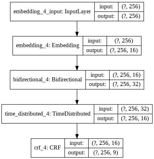
构建模型
模型分为这几层:
-
Embedding 层将词转换成向量,输入为词的索引,输出为词向量
-
max_features: 特征维度(即词汇表大小)
-
embedding_size: 词向量维度(即输出维度)
-
input_length: 输入序列的长度,这里为每个句子的长度(所有句子都填充到一个长度)
-
mask_zero: 让索引 0 不位于词汇表中
-
-
双向LSTM:Bidirectional 双向循环神经网络,输入为一个序列,输出为一个序列
-
hidden_size: 隐藏层维度
-
return_sequences: 是否返回序列,返回序列输出为 (batch_size, timesteps, output_dim) 这里 return_sequences=True 表示返回每个时刻的输出到下一个时刻
-
recurrent_dropout: 添加 dropout 缓解过拟合
-
-
TimeDistributed 层
- 其实就是添加一个全连接层,用于提高模型的质量。
-
CRF 层:CRF 即条件随机场,核心作用是建立状态转移关系
-
units 是第一个参数,表示状态空间的维度,因为我们的不同 TAG 对应不同的状态,所以这里是 TAG 的长度
-
sparse_target 独热编码
-
Embedding Size 为 16,为 max_features 开根的来。max_features 大小即 256.
Hidden Size 为 16,与 Embedding Size 相同。
 1from keras_contrib.layers import CRF
 2
 3
 4def build_model(max_features, max_sentence_len,num_tag, embedding_size, hidden_size):
 5    """
 6    构建模型
 7    """
 8    model = Sequential()
 9
10    # 嵌入
11    # Embedding 层将词转换成向量,输入为词的索引,输出为词向量
12    # - max_features: 特征维度(即词汇表大小)
13    # - embedding_size: 词向量维度(即输出维度)
14    # - input_length: 输入序列的长度,这里为每个句子的长度(所有句子都填充到一个长度)
15    # - mask_zero: 让索引 0 不位于词汇表中
16    model.add(Embedding(max_features, embedding_size, input_length=max_sentence_len))
17
18    # 双向LSTM
19    # Bidirectional 双向循环神经网络,输入为一个序列,输出为一个序列
20    # - hidden_size: 隐藏层维度
21    # - return_sequences: 是否返回序列,返回序列输出为 (batch_size, timesteps, output_dim)
22    #                     这里 return_sequences=True 表示返回每个时刻的输出到下一个时刻
23    # - recurrent_dropout: 添加 dropout 缓解过拟合
24    model.add(Bidirectional(LSTM(hidden_size, return_sequences=True, recurrent_dropout=0.1)))
25
26    # TimeDistributed 层
27    # 其实就是添加一个全连接层
28    model.add(TimeDistributed(Dense(hidden_size, activation="relu")))
29
30    # CRF 层
31    # CRF 即条件随机场,核心作用是建立状态转移关系
32    # - units 是第一个参数,表示状态空间的维度,因为我们的不同 TAG 对应不同的状态,所以这里是 TAG 的长度
33    # - sparse_target 独热编码
34    crf_layer = CRF(num_tag, sparse_target=True)
35    model.add(crf_layer)
36    # 模型编译
37    model.compile(loss=crf_layer.loss_function, optimizer='adam', metrics=[crf_layer.accuracy])
38
39    return model
40
41max_sentence_len = max([len(x) for x in X_train])
42
43# 根据此文的说法 [embedding的size是如何确定? - 知乎](https://www.zhihu.com/question/283167457)
44# 一般采用个经验值,假如 embedding 对应的原始feature的取值数量为 n ,那么我一般会采用 log_2(n) 或者 k n^{1/4}
45# 来做初始的 size,然后 2 倍扩大或缩小,实验几次,一般就能得到一个相对较好的值。
46embedding_size = 16
47hidden_size = 16
48model = build_model(len(word2idx), max_sentence_len, len(tag2idx), embedding_size, hidden_size)
49
50# 显示模型概况
51model.summary()
52tf.keras.utils.plot_model(model, show_shapes=True)
训练和评估
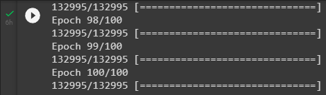
批大小为 8192,代数为 100.
1BATCH_SIZE=8192 # 训练很慢,所以提高批次大小
2EPOCHS=100 # 训练代数
3history = model.fit(X_train, y_train, batch_size=BATCH_SIZE, epochs=EPOCHS, validation_split=0.05)
4
5# 按时间保存
6import time
7timestr = time.strftime("%Y%m%d-%H%M%S")
8model.save(f"drive/MyDrive/ner_model_{timestr}.keras")
六个小时后训练结束。
简单评估一下模型
1results = model.evaluate(X_test, y_test)
2print("test loss, test acc:", results)
15555/15555 [==============================] - 37s 2ms/step
test loss, test acc: [0.023611143523567794, 0.9909988641738892]
可见,在测试集上的准确率达到了 99.1%. Loss 为 0.024 左右。
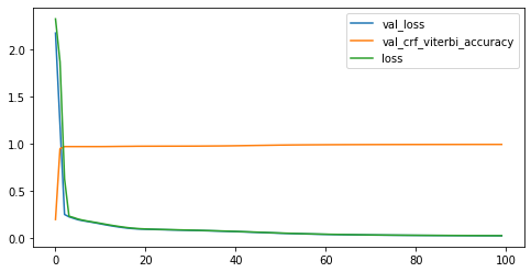
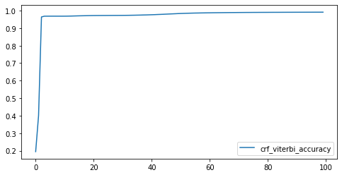
相关指标变化
我们尝试了小样本训练和大样本训练,并且比较了不同的训练代数。
简单来说,小样本训练虽然曲线比较好看,但标注效果很差,基本全标注为 O.
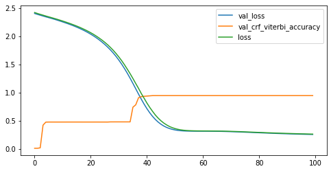
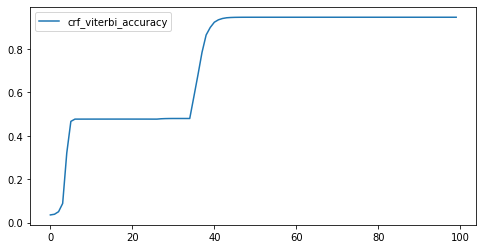
大样本训练:可以看到 Loss 迅速下降。最后精确度达到 99%.
对未知样本进行预测
下面针对未经训练过的样本 test.txt 进行预测。
 1# 正式开始作业任务
 2homework_path = prepare_file("data/test.txt", remote='drive/MyDrive/data/bilstm/test.txt')
 3sentences_raw = open(homework_path, "r").read().split("\n")
 4print("max_sentence_len=",max_sentence_len)
 5print(f"load {len(sentences_raw)} lines")
 6sentences, sentences_break_index = break_sentence(sentences_raw, max_sentence_len)
 7X_homework = [[word2idx.get(w, 0) for w in sentence.split()] for sentence in sentences]
 8
 9# 转换为 np 数组
10X_homework = np.array(X_homework)
11
12# 打印数据概况
13print("Data overview:\n")
14print(f"X_homework: {X_homework.shape}\n")
15
16print("X_homework encoded", X_homework)
17# 填充末尾
18from keras.preprocessing.sequence import pad_sequences
19X_homework = pad_sequences(maxlen=max_sentence_len, sequences=X_homework, padding="post", value=0)
20print("X_homework padded", X_homework)
21y_homework = model.predict(X_homework)
22print(y_homework)
23# 将其转换为 index
24y_homework = np.argmax(y_homework, axis=2)
25# 将 index 转换为 tag
26y_homework = [[idx2tag[i] for i in tag_ids] for tag_ids in y_homework]
27# 将每一行的 tag 列表空格合并
28y_homework = [" ".join(tag_ids) for tag_ids in y_homework]
29# 还原为原始长度
30y_homework_restored = restore_sentence(y_homework, sentences_break_index)
31# 确保还原长度相同
32assert len(y_homework_restored) == len(sentences_raw), "failed to restore"
33# 裁剪多余的填充
34for i, tagline in enumerate(y_homework_restored):
35    y_homework_restored[i] = tagline[:len(sentences_raw[i])]
36# 逐行保存到文件
37with open("test_TAG.txt", "w") as f:
38    for i, tagline in enumerate(y_homework_restored):
39        f.write(tagline + "\n")
40print("preview:")
41print(y_homework_restored[0:5])
整体来说分为这么几步:
-
加载数据。
-
切割,让过长的行转到下一行。
-
对句子进行编码。编码使用的是之前的词典。对于未知词,使用 0 表示。
-
对结尾剩余区域填充。填充到之前规定的最大长度。即 256.
-
预测。调用
model.predict函数,使用之前训练的模型。 -
将预测结果解码。通过
idx2tag词典解码。 -
根据切割点还原。通过
sentences_break_index还原。 -
裁剪多余的填充。根据
sentences_raw也即原始数据的长度裁剪。 -
还原。根据
sentences_break_index即切割点的索引,还原到正确的输出格式。
max_sentence_len= 256
load 26265 lines
/usr/local/lib/python3.7/dist-packages/ipykernel_launcher.py:10: VisibleDeprecationWarning: Creating an ndarray from ragged nested sequences (which is a list-or-tuple of lists-or-tuples-or ndarrays with different lengths or shapes) is deprecated. If you meant to do this, you must specify 'dtype=object' when creating the ndarray.
  # Remove the CWD from sys.path while we load stuff.
Data overview:

X_homework: (32838,)

X_homework encoded [list([135, 306, 31, 830, 31, 407, 831, 60, 108, 178, 1205, 537, 495, 2456, 532, 543, 56, 750, 1524, 11, 2456, 532, 1205, 537, 850, 698, 16, 785, 527, 340, 344, 663, 627, 1135, 32, 32, 824, 32, 885, 6, 49, 850, 698, 1135, 311, 747, 244, 1897, 831, 65, 29, 830, 758, 831, 11, 571, 344, 663, 627, 1135, 31, 824, 208, 885, 6, 11, 2456, 532, 118, 697, 521, 185, 183, 532, 661, 940, 1587, 439, 541, 37, 244, 1205, 70, 2456, 532, 56, 697, 521, 2166, 2741, 4264, 439, 541, 37, 399, 161, 571, 86, 501, 818, 161, 64, 49])
 list([16, 785, 527, 340, 11, 244, 1205, 2456, 532, 118, 56, 556, 697, 279, 627, 1135, 399, 161, 31, 758, 351, 11, 423, 92, 29, 351, 65, 239, 697, 877, 1135, 49, 2456, 532, 56, 556, 697, 279, 627, 1135, 399, 161, 32, 493, 351, 82, 835, 331, 31, 407, 351, 70, 877, 1135, 31, 26, 351, 11, 423, 92, 816, 352, 697, 279, 877, 1135, 31, 493, 351, 11, 816, 369, 697, 279, 877, 1135, 31, 32, 824, 407, 351, 112, 49, 82, 542, 1209, 933, 135, 306, 78, 566, 2644, 112])
 list([2648, 474, 900, 163, 833, 11, 347, 955, 1506, 161, 56, 108, 1005, 11, 347, 955, 509, 151, 180, 993, 98, 91, 185, 282, 108, 439, 1743, 2274, 1191, 481, 11, 91, 1065, 669, 185, 282, 34, 35, 1598, 279, 899, 996, 369, 11, 180, 993, 98, 1021, 657, 697, 1506, 161, 56, 49, 5, 1524, 11, 65, 668, 681, 16, 785, 566, 565, 11, 347, 955, 509, 439, 571, 91, 16, 785, 527, 340, 11, 362, 151, 509, 151, 180, 993, 98, 60, 244, 1005, 335, 279, 1191, 481, 11, 65, 16, 785, 37, 58, 362, 785, 279, 402, 681, 1307, 569, 1719, 405, 49, 82, 135, 306, 366, 16, 2023, 112])
 ...
 list([412, 755, 1657, 11, 697, 344, 743, 412, 679, 49, 137, 48, 11, 595, 1254, 733, 137, 86, 878, 2373, 201, 49, 477, 368, 367, 352, 37, 601, 555, 11, 652, 428, 1167, 540, 187, 621, 65, 103, 142, 779, 1264, 11, 461, 423, 86, 652, 244, 2785, 545, 195, 865, 214, 1216, 49, 85, 246, 733, 86, 91, 137, 764, 1755, 37, 290, 817, 108, 11, 454, 762, 845, 280, 11, 335, 576, 616, 617, 679, 142, 807, 660, 49])
 list([2648, 291, 9, 135, 306, 71, 1349, 1748, 1279, 535, 1323, 1666, 29, 493, 30, 1666, 31, 758, 758])
 list([])]
X_homework padded [[ 135  306   31 ...    0    0    0]
 [  16  785  527 ...    0    0    0]
 [2648  474  900 ...    0    0    0]
 ...
 [ 412  755 1657 ...    0    0    0]
 [2648  291    9 ...    0    0    0]
 [   0    0    0 ...    0    0    0]]
[[[1. 0. 0. ... 0. 0. 0.]
  [1. 0. 0. ... 0. 0. 0.]
  [0. 1. 0. ... 0. 0. 0.]
  ...
  [1. 0. 0. ... 0. 0. 0.]
  [1. 0. 0. ... 0. 0. 0.]
  [1. 0. 0. ... 0. 0. 0.]]

 [[1. 0. 0. ... 0. 0. 0.]
  [1. 0. 0. ... 0. 0. 0.]
  [1. 0. 0. ... 0. 0. 0.]
  ...
  [1. 0. 0. ... 0. 0. 0.]
  [1. 0. 0. ... 0. 0. 0.]
  [1. 0. 0. ... 0. 0. 0.]]

 [[0. 1. 0. ... 0. 0. 0.]
  [0. 0. 1. ... 0. 0. 0.]
  [0. 0. 1. ... 0. 0. 0.]
  ...
  [1. 0. 0. ... 0. 0. 0.]
  [1. 0. 0. ... 0. 0. 0.]
  [1. 0. 0. ... 0. 0. 0.]]

 ...

 [[1. 0. 0. ... 0. 0. 0.]
  [1. 0. 0. ... 0. 0. 0.]
  [1. 0. 0. ... 0. 0. 0.]
  ...
  [1. 0. 0. ... 0. 0. 0.]
  [1. 0. 0. ... 0. 0. 0.]
  [1. 0. 0. ... 0. 0. 0.]]

 [[1. 0. 0. ... 0. 0. 0.]
  [1. 0. 0. ... 0. 0. 0.]
  [1. 0. 0. ... 0. 0. 0.]
  ...
  [1. 0. 0. ... 0. 0. 0.]
  [1. 0. 0. ... 0. 0. 0.]
  [1. 0. 0. ... 0. 0. 0.]]

 [[1. 0. 0. ... 0. 0. 0.]
  [1. 0. 0. ... 0. 0. 0.]
  [1. 0. 0. ... 0. 0. 0.]
  ...
  [1. 0. 0. ... 0. 0. 0.]
  [1. 0. 0. ... 0. 0. 0.]
  [1. 0. 0. ... 0. 0. 0.]]]
preview:
[
    'O O B_T I_T I_T I_T I_T O B_LOC I_LOC O O O B_LOC I_LOC I_LOC O O O O B_LOC I_LOC O O O O O O O O O O O O O O O O O O O O O O O O O O O O B_T I_T I_T I_T O O O O O O O O O O O O B_LOC I_LOC I_LOC O O B_LOC',
    'O O O O O O O B_LOC I_LOC I_LOC O O O O O O O O O O O O O O O O O O O O O O B_LOC I_LOC O O O O O O O O O O O O O O O O O O O O O O O O O O O O O O O O O O O O O O O O O O O O O O O O O',
    'B_T I_T I_T I_T I_T O B_LOC I_LOC O O O O O O B_LOC I_LOC O O O O O O O O O O O O O O O O O O O O O O O O O O O O O O O O O O O O O O O O O O O O O O O O O B_LOC I_LOC O O O O O O O O O O O O O O O O O O O O O O O O O O O O O',
    'O O B_T I_T O B_LOC I_LOC I_LOC O O O O O O B_T I_T O O O O O O O O O O O O O O O O O O O O O O O O O O O O O O O O O O O O O O O O O O O O O O O O O O O O O O O O O O O O O O O O O O O O O O O O O O O O O O O O O O O O O O O O O O O O O O O O O O O B_T I_T I_T I_T I_T O O O O O O O O O O O O O O O O',
    'O O O O B_T I_T I_T I_T I_T O B_LOC I_LOC I_LOC O O O O O O O O O O O O O O O O O O O O O O O O O O O O O O O O O O O O O O O O O O O O O O O O O O O O O O O O O O O O O O O O O O O O O O O O O O O O O O O O B_LOC I_LOC I_LOC I_LOC O O O O B_LOC I_LOC O O O O O O B_LOC I_LOC O O O O O B_LOC I_LOC O O O O O O O B_PER I_PER I_PER O O O O O O O O O O O O O O O O O O O O O O O O O O O O O O'
]
对比 test.txt 的内容:
记 者 1 月 1 5 日 从 上 海 铁 路 局 淮 南 西 站 获 悉 , 淮 南 铁 路 预 计 春 运 期 间 发 送 旅 客 3 3 . 3 万 人 。 预 计 客 流 最 高 峰 日 为 2 月 6 日 , 将 发 送 旅 客 1 . 8 万 人 , 淮 南 东 开 往 广 州 南 及 北 京 方 向 的 高 铁 、 淮 南 站 开 往 沪 杭 甬 方 向 的 列 车 将 是 热 门 车 次 。
春 运 期 间 , 高 铁 淮 南 东 站 共 开 行 旅 客 列 车 1 6 对 , 其 中 2 对 为 增 开 临 客 。 淮 南 站 共 开 行 旅 客 列 车 3 4 对 ( 图 定 1 5 对 、 临 客 1 9 对 , 其 中 节 前 开 行 临 客 1 4 对 , 节 后 开 行 临 客 1 3 . 5 对 ) 。 ( 江 劲 松 记 者 张 安 浩 )
[ 今 天 下 午 , 合 肥 火 车 站 上 空 , 合 肥 警 用 直 升 机 在 广 场 上 方 盘 旋 巡 逻 , 在 绕 着 广 场 连 续 飞 行 几 圈 后 , 直 升 机 才 离 开 火 车 站 。 据 悉 , 为 确 保 春 运 安 全 , 合 肥 警 方 将 在 春 运 期 间 , 利 用 警 用 直 升 机 从 高 空 进 行 巡 逻 , 为 春 运 的 顺 利 运 行 “ 保 驾 护 航 ” 。 ( 记 者 项 春 雷 )
记 者 日 前 从 安 徽 省 商 务 厅 获 悉 , 去 年 以 来 , 境 外 世 界 5 0 0 强 企 业 在 皖 踊 跃 设 立 新 项 目 , 投 资 呈 现 较 快 增 长 态 势 。 据 省 商 务 厅 统 计 , 全 年 共 新 批 境 外 世 界 5 0 0 强 企 业 投 资 企 业 1 7 个 , 同 比 增 长 3 0 . 8 % , 合 计 投 资 总 额 5 . 6 亿 美 元 , 合 同 外 资 2 亿 美 元 。 截 至 去 年 1 2 月 底 , 共 有 6 7 家 境 外 世 界 5 0 0 强 在 安 徽 省 投 资 设 立 了 1 0 5 家 企 业 。
据 介 绍 , 2 0 1 3 年 , 安 徽 省 立 足 主 导 产 业 、 紧 扣 本 地 首 位 产 业 , 突 出 产 业 链 条 补 足 和 延 伸 , 切 实 转 变 招 商 引 资 方 式 , 着 力 打 造 产 业 配 套 、 自 主 创 新 等 招 商 引 资 新 优 势 。 全 年 新 引 进 境 外 世 界 5 0 0 强 4 家 , 分 别 是 西 班 牙 国 家 银 行 、 法 国 威 立 雅 水 务 、 台 湾 鸿 海 精 密 和 英 国 利 洁 时 。 同 时 , 卡 特 彼 勒 、 西 门 子 、 菲 亚 特 、 三 菱 电 机 、 麦 德 龙 、 欧 尚 、 华 润 等 已 来 投 资 5 0 0 强 企 业 增 设 项 目 1 3 个 , 合 计 投 资 总 额 3 . 1 亿 美 元 , 合 同 外 资 1 . 1 亿 美 元 。
可以看到长度一致,并且 1 月 1 5 日,上 海,淮 南 西,3 0 . 8 % 等序列均被正确标注。
总结
限于训练时间太久,没有采用所有数据集进行多批次的训练。但从结果来看,由于对数据进行了较好的预处理,效果还是可以的。